December
1974 – November 1981
by
Hamish Lindsay

Honeysuckle Creek tracked the two Helios spacecraft throughout its Deep Space
life, in fact one of our last tracks was of Helios 1, which was launched on 10
December 1974, around about the time we joined the Deep Space Network. We spent
countless hours tracking the two Helios spacecraft.
We
had to modify the antenna to accommodate the Helios signals. Neil Sandford developed
a grid to cover the feedcone window, opened and closed remotely from the servo
console. If the servo operator forgot to open the grid for the other spacecraft,
or forgot to close it for Helios, the signal was degraded by about 3db.
|
Paul Mullen at Honeysuckle’s servo console.
A polariser was installed on the feedcone to support Helios, and there’s a reference to it on the console in front of Paul.
Photo: Hamish Lindsay. 5x4 inch negative from the Tidbinbilla archives. 2024 scan: Colin Mackellar. |
Helios 1 and Helios 2 were a pair of deep space probes developed by
the Federal Republic of Germany (FRG) in a cooperative program with NASA. Ten
experiments were provided by scientists from both FRG and the USA. NASA supplied
the Titan/Centaur launch vehicle. Each spacecraft was equipped with two booms
and a 32-metre electric dipole. The purpose of the mission was to make pioneering
measurements of the interplanetary medium from the vicinity of the earth's orbit
to 0.3 AU. The spin axis was normal to the ecliptic, and the nominal spin
rate of the spacecraft was 1 revolution per second.
HELIOS
1 was launched on 10 December 1974, and HELIOS 2 on 15 January 1976. Both were
placed in elliptical orbits about the Sun with their perihelions well within
the orbit of Mercury, aphelions at the orbit of Earth, with orbital periods
of about 190 days.
What
made the two Helios missions so unusual was that the two spacecraft made incredibly
close passes to the Sun resulting in very high orbital speeds. These high speeds
resulted from the fact that both probes were placed into very elliptical orbits
around the Sun. When a probe is placed into a circular orbit, its speed remains
a constant. When in a highly elliptical orbit, however, a vehicle will reach
very high speeds when it is close to the body it is orbiting but slow down considerably
when it is far away.
The
Helios missions both orbited in this manner, with a furthest distance (or aphelion)
of nearly 1 Astronomical Unit (AU), which is the distance at which the Earth
orbits the Sun. Meanwhile, the closest approach (or perihelion) of the Helios
probes was about 0.3 AU, closer than any spacecraft had been at the time. The
eccentricity of such an orbit is about 0.54 with a period of about 190 days.
HELIOS
2 IS THE FASTEST MAN-MADE OBJECT.
The
maximum speed of Helios 2, which achieved its perihelion distance of 0.29 AU
on 17 April 1976, is quoted as about 241,350 kilometres per hour. For comparison,
the aphelion speed of Helios 2 turns out to be only 72,985 km/h at its farthest
distance of 0.983 AU. This massive differential between the vehicle’s maximum
and minimum speeds graphically illustrates how much an elliptical orbit varies
from the circular orbit discussed earlier.
The
reason the Helios probes were given such unusual orbits is that they were intended
to make various measurements of the interplanetary medium between the Sun and
Earth. Each probe was equipped with 10 experiments including high-energy particle
detectors to measure the solar wind, magnetometer readings of the Sun's magnetic
field, measurements of variations in electric and magnetic waves, and a micrometeoroid
experiments. The two probes completed their primary missions by the early 1980s
but were still sending data as late as 1985. Though they are no longer functional,
both craft remain in their eccentric orbits around the Sun.
Here
is a brief summary of the experiments carried by the Helios spacecraft:
1.
Plasma Experiment
The
plasma experiment was the responsibility of the Max-Planck-Institut für
Physik und Astrophysik of Munich. It consisted of four independent instruments
designed to investigate the solar wind plasma. The bulk velocity, density, and
temperatures of the different particles were measured. By measuring the velocity
distribution functions of the different kinds of particles, the all-important
hydrodynamic parameters of the solar wind plasma can be derived. Three instruments
analysed the positive components (protons and heavier ions with energy-per-charge
values from 0.155 to 15.32 kV) of the solar wind. Two of them allowed for
an angular resolution in both directions of incidence. One instrument measured
electrons in the energy range from 0.5 the 1660 eV with one-dimensional
angular resolution.
2
and 3. Flux-gate Magnetometers
The
Institut für Geophysik und Meteorologie der Universität Braunschweig
in Germany, the Goddard Space Flight Center in Maryland USA, and Istituto di
Fisica, Università di Rome were responsible for the magnetometers, which
measured the field strength and direction of low frequency magnetic fields in
the Sun’s environment. These fields are extended outwards into space by
the solar wind in a spiral direction. The main components are in the ecliptic
plane. The Förstersonden flux-gate magnetometer experiments used triaxial,
orthogonal flux-gate sensors mounted on a boom extending about 2 metres
from the spacecraft. The bandwidth is 4 Hz. Two measuring ranges are used
with automatic switching. The sensitivity range extends from -100 nT to
+100 nT.
4.
Search Coil
Magnetometer
In
the interplanetary plasma, besides stationary plasma and slowly varying magnetic
fields, components of higher frequencies can be found. This experiment complements
the measuring range of Experiments 2 and 3 so that the magnetic fields can be
measured between 0 and 3 kHz. The object of this experiment is to measure and
analyse rapidly fluctuating disturbances and shock waves. Mounted on the end
of the 2-metre boom with Experiments 2 and 3, three coils are mounted perpendicular
to each other to measure the three components of the magnetic field. The Institut
für Nachrichentechnik und Institut für Geophysik und Meteorologie,
University of Braunschweig in Germany provided this experiment.
5.
Plasma Wave Experiment
NASA’s
Goddard Space Flight Center, the University of Minnesota and the University
of Iowa’s plasma wave experiment utilized the 32-metre tip-to-tip dipole
antenna to detect the electric component of plasma waves.
This
summary of results from the HELIOS plasma wave experiment demonstrates that
this investigation has produced many important new results over the 10 year
period since HELIOS 1 was launched. This investigation confirmed a basic theory
for the generation of type III radio bursts that was first proposed over 20
years ago, and it revealed the existence of enhanced levels of ion acoustic
wave turbulence in the solar wind. The long duration of the observations and
the extended radial distance coverage provided a vast quantity of data on the
temporal and radial variation of these and other plasma wave phenomena over
almost an entire solar cycle. The results obtained show that the plasma processes
occurring in the solar wind are very complicated and many important questions
still remain to be answered. Hopefully, with the continued operation of HELIOS
1 and further study of the existing data some of these questions can be answered.
6
and 7 Cosmic Radiation Experiments
From
the Galaxy’s billions of stars, the Sun, and from planetary atmospheres
charged particles of high energy move at almost the velocity of light into our
solar system. Consisting mainly of protons, but also of helium and heavier nuclei,
these particles are called cosmic radiation. The cosmic ray particle experiment
(University of Kiel in Germany) consisted of a detector telescope containing
five semiconductor detectors of increasing thickness, a sapphire Cherenkov detector
surrounded by an anticoincidence scintillation detector, and an on-board handling
system. The instrument was capable of measuring protons and heavier nuclei from
1.7 to more than 400 MeV/n and MeV electrons. Experiment 7 also measured
the X-ray intensity of the Sun. NASA’s Goddard Space Flight Center in Maryland
and the Institut für Reine und Angewandte Kernphysik of the University
of Kiel in Germany handled these two experiments.
8 Low-Energy Electron and Ion Spectrometer
Experiment
8 investigated the higher energy portion of the crossover region between the
solar wind particles and the cosmic rays. The spectrometer utilizes an inhomogenous
magnetic field for separation of charged particles. Protons (and heavier particles)
traversed the magnetic field almost unaffected and were detected in a telescope
arrangement consisting of two semiconductor detectors. Electrons were focussed
and detected by four semiconductor detectors. Positrons (if present) were deflected
in the opposite direction and detected in another detector. The Max-Planck-Institut
für Aeronomie, Kaltenburg-Lindau in Germany provided this experiment.
Zodiacal
Light Photometer
The
weak glow in the sky, called the Zodiacal Light, has been known for a long time.
It is the result of the scattering of sunlight by interplanetary dust particles.
The density and distribution of these particles cannot be measured from Earth
so Helios measured the intensity of the light at angles of 15 degrees, 30 degrees,
and 90 degrees with respect to the ecliptic. The photometers scanned through
a full circle on each rotation of the spacecraft. The intensity of the unfiltered
light was measured in three wavelength ranges, 360, 420 and 530 nm. Polarisers
could be introduced to determine the polarisation index of the zodiacal light.
Responsibility
for this experiment lay with the Max-Planck-Institut für Astronomie and
the Landessternwarte Heidelberg-Königsstuhl in Germany.
Micrometeoroid
Analyser
Until
Helios the characteristics of micrometeoroids had not been investigated to any
great extent. Helios investigated the composition, charge, mass, velocity and
direction of interplanetary dust particles. Comets have known to be the source
of interplanetary dust. The Max-Planck-Institut für Kernphysik in Heidelberg,
Germany provided this experiment.
 |
|
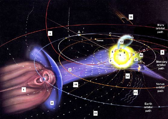
Perspective
view of the solar system, not to any scale, and the Earth’s magnetosphere
and the Sun’s features are greatly simplified and magnified to show
them clearly.
Helios
1 was launched from Earth at the position marked ‘A’ and its
orbital path is shown in white. The Earth and Venus are shown when Helios
reached its closest approach to the Sun the first time. Mercury at the
same time is shown just below Helios.
There
was a blackout period when Helios passed behind the Sun, shown between
points ‘B’ and ‘C’.
1.
The Earth’s magnetosphere is shown
streaming away from the Sun.
2.
The Earth’s shock front. These two
features are formed by the interaction between the Earth’s magnetic
field and the solar wind passing by.
3.
The Solar Wind originates from the hot
Corona and travels at speeds of up to 1,800,000 kilometres per hour. It
is not uniform as it is affected by magnetic clouds, interacting regions,
and composition variations. If a slow moving stream of solar wind is overtaken
by a faster moving stream the resulting interaction produces shock waves
that can accelerate particles to extremely high speeds. It streams out
like the water from a lawn sprinkler as the Sun spins on its axis every
27 Earth days.
4.
Sunspots on the surface of the Sun. Sunspots
have been known to exist since the invention of the telescope - Galileo
is often quoted as one of the first to refer to them around 1610. Sunspots
are thought to be the result of pent-up magnetic fields below the surface
of the Sun breaking through making relatively cool areas when new hot
gas is inhibited from reaching the surface. Sometimes larger than the
Earth, they can be in groups, and last for weeks to months, depending
upon their size. They do not appear randomly over the surface - they are
concentrated above and below the solar equator. Spots that appear in the
northern hemisphere are mirrored in the southern hemisphere, mostly in
pairs, the leading spot carrying the opposite polarity to the trailing
spot. Sunspots are linked to the Sun’s magnetic activity, their number
rising and falling over 11 year cycles, called the Solar Cycle.
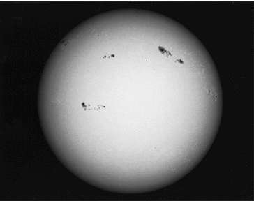
Sunspots under
white light.
5.
Long Filaments stretching out from the surface of
the Sun. Filaments are long, thin regions of relatively cool
gases stretching 100,000 kilometres out from the surface, held in place
by magnetic fields above the chromosphere. They can last weeks, or months
before dropping back to be absorbed back into the Sun’s surface.
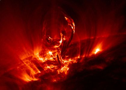
A
Filament photographed by the satellite TRACE.
6.
The hot Corona is grouped into three types, the White Light
Corona, Emission Line Corona, and X-Ray Corona. The Corona is the upper
atmosphere of the Sun and can only be seen during total eclipses or with
the use of special equipment as it is a million times darker than the
Photosphere.
 
The
left image during a solar eclipse in 1980, near solar maximum activity,
shows streamers all around the disc, while the right image taken in
1988, near minimum activity shows large bottle shaped streamers concentrated
at the equator.
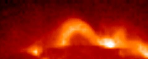
7.
Coronal arches are fountains of hot gases stretching 480,000
kilometres above the surface. They heat up as they rise through the first
16,000 kilometres, flow along the magnetic lines and cool down as they
stream back into the surface at more than 360,000 kilometres per hour.
Millions of different sized arches make up the corona.
8.
Streamers of magnetic loops extending between areas of opposite
magnetic polarity. Streamers and loops are hot gases trapped in magnetic
field lines up to 800,000 kilometres long. They emanate from constantly
changing north and south poles scattered all over the surface. The magnetic
fields are believed to originate from a region 220,000 kilometres below
the surface which scientists believe is the source of all magnetism in
the Sun.
9.
The Coronal arches can continue into
boundary regions in the interplanetary magnetic field.
10.
The Interplanetary Magnetic Field, also
called the IMF. Originating from the Sun the IMF spirals out (called the
Parker Spiral) carried by the solar wind through the heliosphere to eventually
reach Interstellar Space beyond the planet Pluto.
11.
Alfven waves and shock
waves (12) produced during flares on the Sun can cause kinks
in the Sun’s magnetic field. Like the movement of a plucked guitar
string, they travel down the Sun’s magnetic field, embedding in the
solar wind to eventually cause auroras on Earth. They are named after
Hannes Alfven who discovered them in 1942.
13.
During flare eruptions, radio waves and
X-ray waves occur when charged particles are accelerated to high energies.
14.
The propagation of ‘solar radiation’ takes place in the Corona’s magnetic fields and in the spiral paths
around the interplanetary magnetic field. Solar radiation is the electromagnetic
radiation (light energy) transmitted into space in units of photons. Without
this radiation life on Earth would not exist. It is over 9 KW/metre squared
at Mercury, dropping to about 1.6 KW/metre squared at Earth to almost
0 at Saturn. Roughly half the radiation that reaches the Earth’s
upper atmosphere reaches the surface.
15.
Galactic cosmic radiation constantly
penetrates into the interplanetary medium from outside the solar system.
16.
The scattering of sunlight on small dust
particles in space produces the Zodiacal Light. These dust particles are
released into the interplanetary medium by comets and small asteroids.
The smaller particles are blown away by the solar wind but the larger
particles, 0.1 to 100 micrometre, spiral in to the Sun and form a flattened
disc around it in the ecliptic plane, visible from the Earth under certain
conditions.
17.
Zodiacal Light may be regarded as a continuation of part of
the Sun’s low-intensity Corona. |


